
Elasticsearch in Production: The Definitive Architecture & Operations Guide

Definition
Elasticsearch is a distributed, RESTful search and analytics engine capable of solving a growing number of use cases. At its core, it is a NoSQL database, but unlike traditional databases designed for storage and retrieval, Elasticsearch is optimized for speed and relevance.
Architecture & Capacity Planning
This diagram illustrates a typical producción cluster architecture, showing the separation of duties between dedicated master nodes, tiered data nodes (hot/warm), and coordinating nodes.

1. Node Roles
A. Mandatory Basic Roles
1. Master-eligible node (master)
Function: Responsible for cluster-wide actions such as creating or deleting indices, tracking which nodes are part of the cluster, and allocating shards to nodes.
Why it's mandatory: Without a master, the cluster cannot be formed, and no cluster-level changes can be tracked.
Production Tip: You typically need 3 dedicated master nodes for High Availability (to avoid "split-brain").
2. Data node (data)
Function: Holds the shards that contain your indexed documents. These nodes perform data-related operations like CRUD, search, and aggregations.
Why it's mandatory: Without data nodes, you cannot store any data.
Sub-roles (Tiered Architecture):
data_content: For general-purpose data that doesn't fit a time-series lifecycle.data_hot: For strictly time-series data (e.g., logs) that is being actively written to and queried.data_warm: For older data that is read-only but still queried frequently.data_cold: For data accessed infrequently (optimized for storage).data_frozen: For data stored in object storage (S3) and rarely queried (Searchable Snapshots).
B. Core Utility Roles (Highly Recommended)
While not strictly "mandatory" for the cluster to start, these are standard in almost all production environments.
1. Ingest node (ingest)
Function: Runs "ingest pipelines" to pre-process documents before indexing. This acts like a lightweight Logstash inside Elasticsearch (e.g., parsing JSON, removing fields, renaming fields).
Default Behavior: Every node is an ingest node by default unless configured otherwise.
2. Coordinating-only node (No specific role set)
Function: These nodes have an empty role list (
node.roles: []). They act as "Smart Load Balancers." They accept search requests, distribute them to the specific data nodes holding the data, gather the results, perform the final reduction (sorting/aggregating), and send the response to the client.Use Case: Large clusters with heavy search traffic to prevent data nodes from being overwhelmed by CPU-intensive aggregation tasks.
C. Specialized Roles (Optional)
These are specific to certain features of the Elastic Stack.
1. Machine Learning node (ml)
Function: Runs the native Machine Learning jobs (anomaly detection, forecasting).
Requirement: These jobs are CPU and RAM intensive. If you use ML features, you must have at least one ML node.
2. Remote Cluster Client (remote_cluster_client)
Function: Allows the cluster to connect to other clusters (Cross-Cluster Search or Cross-Cluster Replication).
Default: Enabled by default on all nodes.
3. Transform node (transform)
- Function: Runs transform jobs which pivot or summarize data into new indices (similar to "Materialized Views" in SQL).
4. Voting-only node (voting_only)
Function: A master-eligible node that can participate in master elections (voting) but cannot actually become the elected master.
Use Case: Rarely used; mostly for tie-breaking in even-numbered clusters.
2. Hardware Requirements
These figures are based on the constraints of the JVM (Java Virtual Machine) and operational best practices for recovery and stability.
A. RAM (Memory)
This is the most critical resource. It is split between the JVM Heap (for the application) and the OS Filesystem Cache (for Lucene segment files).
Minimum:
8 GB-16 GB- Running a production node with less than 8GB is risky. You need enough headroom for the OS to cache frequently accessed index segments.
The "Sweet Spot":
64 GB- This is the standard specification for a high-performance node. It allows you to allocate ~30GB to the Heap and leave ~34GB for the OS cache.
Maximum (Effective):
64 GB(Physical RAM)
⚠️ The "Compressed Oops" Limit
You should strictly avoid allocating more than 31GB-32GB to the JVM Heap. If the Heap crosses ~32GB, the JVM stops using "Compressed Object Pointers" (pointers swell from 32-bit to 64-bit). This drastically reduces memory efficiency, effectively cutting your available memory by half.
B. Disk (Storage)
Disk speed dictates indexing throughput, and disk size dictates how long recovery (rebalancing shards) takes.
Type Requirement: SSD / NVMe
- Spinning HDDs are only acceptable for "Cold" or "Frozen" tiers.
Minimum Capacity:
200 GB- Small clusters need enough space for logs, the OS, and headroom for shard merging.
Maximum Capacity (Per Node):
Hot Nodes (High IO):
2 TB-4 TBlimit.- Reasoning: If a node holds 10TB of hot data and dies, replicating that 10TB to a new node over the network takes hours or days, leaving the cluster in a "Yellow" (at risk) state.
Warm/Cold Nodes:
10 TB-16 TB.- Reasoning: Since these nodes are query-heavy but low-write, you can pack them with dense storage, provided you accept slower recovery times.
C. Network
Elasticsearch is a distributed system; the network is the bus.
Minimum:
1 Gbps(Gigabit Ethernet)Acceptable only for small clusters with low indexing rates.
Risk: During a "peer recovery" (when a node comes back online), a 1 Gbps link will be 100% saturated, causing search latency to spike.
Recommended / Maximum:
10 Gbps-25 Gbps- 10 Gbps is the standard for modern production clusters to ensure recovery doesn't impact live traffic.
Latency: Must be low single-digit ms (intra-datacenter).
- Warning: Spanning a single cluster across distinct geographical regions (e.g., US-East to EU-West) is generally unsupported and will cause instability due to timeout errors.
3. Sizing & Sharding
This diagram provides a clear visualization of how a single index is divided into primary shards (P) and how each primary shard has a corresponding replica shard (R) distributed across different nodes for high availability.

A. Shard Strategy
Sharding is the mechanism that allows Elasticsearch to scale beyond the hardware limits of a single server. However, it is the most common source of performance issues in production.
1. The Concept
An Elasticsearch index is actually a logical grouping of Shards. Each shard is a self-contained instance of Apache Lucene, which is a fully functional search engine in its own right. When you execute a search on an index, Elasticsearch queries all relevant shards in parallel and merges the results.
2. The "Oversharding" Trap
New users often think, "If shards provide parallelism, more shards must mean more speed." This is a fallacy known as oversharding.
The Metadata Overhead: Every shard consumes resources. The Cluster State (the "brain" of the cluster) must track the location, status, and size of every shard. If you have 100,000 small shards, the Cluster State grows huge, and updates (like creating a new index) become incredibly slow.
The "Map-Reduce" Tax: When you search an index with 50 shards, the coordinating node must send the request to 50 places, wait for 50 responses, and merge 50 results. If those shards are tiny (e.g., 50MB), the overhead of managing the request outweighs the benefit of parallel processing.
Memory Cost: Each shard has a baseline memory footprint in the JVM Heap to hold Lucene segment info. Too many small shards will exhaust your Heap memory even if the cluster is idle.
✅ The Golden Rule: 10GB – 50GB
For general-purpose search (e.g., products, users), aim for a shard size between 10GB and 50GB.
Why > 10GB? To minimize the per-shard overhead and maximize efficient compression.
Why < 50GB? To ensure recovery is fast. If a node fails, moving a 50GB shard to a new node over the network is manageable. Moving a 500GB shard takes so long that your cluster remains in a vulnerable state ("Yellow" health) for hours.
B. Replicas
Replication serves two distinct purposes in a cluster: High Availability (HA) and Read Throughput.
1. Failover (High Availability)
A Replica Shard is a precise copy of a Primary Shard.
The Mechanism: If the node holding a Primary Shard crashes, the master node instantly "promotes" the Replica Shard (living on a different node) to be the new Primary.
Production Standard: You must set
number_of_replicas: 1(at minimum). This ensures that if any single node fails, no data is lost, and the cluster remains fully operational.The Trade-off: Replicas double your storage requirements. 100GB of data with 1 replica requires 200GB of physical disk space.
2. Read Throughput (Scaling Search)
Unlike Primary shards, which handle both reads and writes, Replicas are usually used for reads.
Load Balancing: When a search request comes in, the coordinating node intelligently routes it. It can go to the Primary or any of its Replicas.
Scaling Up: If your application is "Read Heavy" (e.g., an e-commerce site where users search frequently but products change rarely), you can increase performance by adding more replicas.
- Example: An index with 1 Primary and 5 Replicas allows 6 nodes to answer search queries simultaneously for that specific data.
Key Distinction:
Primary Shards are fixed at index creation (changing them requires reindexing).
Replica Shards can be changed dynamically. You can scale from 1 replica to 5 replicas instantly if you expect a traffic spike (like Black Friday), and scale back down afterwards.
Environment Preparation (OS Tuning)
Elasticsearch is sensitive to Operating System configurations. Failing to tune these will often prevent the cluster from starting (Bootstrap Checks).
1. Disable Swapping (The "Performance Killer")
The Concept: In a standard server, if physical RAM is full, the OS moves inactive memory pages to the hard disk (swap space). For Elasticsearch, this is catastrophic. The Java Garbage Collector (GC) needs to scan memory to reclaim space. If that memory is on the disk (which is 100,000x slower than RAM), a GC cycle that usually takes milliseconds will take seconds or minutes.
- The Result: The node becomes unresponsive ("Stop-the-world" pause), the cluster thinks the node is dead, drops it, and triggers a massive data rebalance.
How to configure it
You have two main methods. The best practice is to do both.
OS Level (Permanent): Disable swap completely.
sudo swapoff -aApplication Level (Memory Lock): Force Elasticsearch to lock its memory address space into RAM so the OS cannot swap it out.
In
elasticsearch.yml:bootstrap.memory_lock: trueNote: You may need to edit the systemd service file (
systemctl edit elasticsearch) to allow this limit:[Service] LimitMEMLOCK=infinity
2. File Descriptors (The "Capacity Limit")
The Concept: Elasticsearch (via Lucene) breaks your data into heavily compressed immutable files called "segments." A single node can easily hold thousands of these small files open simultaneously. The default Linux limit for open files per user is often 1024. This is far too low. If Elasticsearch hits this limit, it can silently lose data or crash because it cannot write to new files.
How to configure it
You must increase the limit to at least 65,536.
Check current limit:
ulimit -nPermanent fix: Edit
/etc/security/limits.conf:elasticsearch - nofile 65536(If you install via RPM/Deb package, this is often done automatically, but you must verify it).
3. Virtual Memory (The mmap Requirement)
The Concept: This is specific to how Lucene reads data. It uses a system call called mmap (memory map) to map the files on the disk directly into the virtual memory address space. This is incredibly fast because it lets the kernel manage file caching. However, the default operating system limit on how many "memory maps" a process can own is usually 65,530. Elasticsearch requires significantly more.
How to configure it
This is the most common reason for startup failures.
Command (Live):
sysctl -w vm.max_map_count=262144Permanent fix: Add this line to
/etc/sysctl.conf:vm.max_map_count=262144
4. JVM Heap Size (The Balancing Act)
This is the most misunderstood setting. You are configuring the Java Virtual Machine (JVM) memory.
A. Xms and Xmx (Min vs. Max)
The Problem: By default, Java starts with a small heap (
Xms) and grows it as needed up to the max (Xmx). This resizing process pauses execution.The Fix: Set them to the same value. This allocates all the memory immediately at startup, preventing resizing pauses.
  # /etc/elasticsearch/jvm.options
  -Xms4g
  -Xmx4g
B. The 50% Rule (Why not 100%?)
If you have a 64GB machine, why give Elasticsearch only 30GB? Why not 60GB?
The Reason: Elasticsearch relies on two types of memory:
JVM Heap: For query objects, aggregations, and cluster state.
OS Filesystem Cache: This is where the actual data (Lucene segments) lives.
If you give all RAM to the Heap, the OS has no room to cache the files. The disk will be thrashed, and performance will tank.
Rule: 50% to Heap, 50% left free for the OS.
C. The 32GB Limit (Compressed Oops)
You must never set the Heap above ~32GB (exact threshold varies, usually 30GB-31GB is safe).
The Science: Below 32GB, Java uses "Compressed Ordinary Object Pointers" (Compressed Oops). It uses 32-bit pointers to reference memory.
The Trap: Once you cross the threshold (e.g., 32.1GB), Java switches to 64-bit pointers. These are larger.
The Result: A 35GB Heap actually stores less data than a 31GB Heap because the pointers themselves take up so much more space. Plus, it consumes more CPU bandwidth.
Security (The "Must-Have" Layer)
This section often trips up new administrators because it involves certificates and passwords, which can be tedious. However, in modern Elasticsearch (version 8.x+), security is enabled by default. You cannot run a production cluster without it.
1. TLS/SSL Encryption (The "Encrypted Tunnel")
Encryption prevents "Man-in-the-Middle" attacks. In Elasticsearch, we implement this in two distinct layers. If you miss the first one, your cluster will not even start.
A. Transport Layer (Node-to-Node)
What it is: The internal communication channel on port
9300where nodes talk to each other (electing masters, moving shards, replicating data).Why it's mandatory: Elasticsearch requires mutual trust. Node A must prove to Node B that it is a legitimate part of the cluster, not a rogue server trying to steal data.
The Mechanism:
You generate a Certificate Authority (CA).
You sign a certificate for each node using that CA.
Crucial Note: If you do not enable Transport SSL, Elasticsearch will refuse to bind to a non-loopback IP address (i.e., it stays in "Development Mode").
Key Tool:
bin/elasticsearch-certutil(This built-in tool simplifies creating these certificates).
B. HTTP Layer (Client-to-Cluster)
What it is: The external API on port
9200where Kibana, your application (Java/Python/Node.js), and users connect.Why it's critical: Without this, Basic Auth credentials (username/password) are sent in plain text. Anyone on the network can sniff the admin password.
Configuration: You generally use the same CA to sign these certificates, or you can use a public CA (Let's Encrypt, Verisign) if your cluster is public-facing.
2. Authentication & RBAC (The "Gatekeeper")
Once the connection is secure, you need to control who is logging in and what they can touch. This is Role-Based Access Control (RBAC).
A. The Built-in Users
When you first start the cluster, you run bin/elasticsearch-reset-password. This sets up reserved accounts that are vital for the stack:
elastic: The "Superuser" (Root). It has full control.Danger: Do not use this account in your application code! If those credentials leak, your entire cluster is compromised.
kibana_system: A service account used only by the Kibana server to talk to Elasticsearch. It cannot be used to log in to the dashboard.
B. The Principle of Least Privilege
You should create custom roles for every specific use case.
The "Developer" Role: Can read and monitor indices but cannot delete data or change cluster settings.
The "App" Role: Can write to the
logs-*index but cannot read from thesalary-dataindex.Document Level Security (DLS): You can even restrict access within a single index.
- Example: "User A can search the
employeesindex, but only document wheredepartment: 'marketing'."
- Example: "User A can search the
3. Audit Logging (The "Black Box")
If data disappears or leaks, how do you know what happened?
What it tracks: You can configure it to log specific events: "Authentication Failed," "Index Deleted," or even "User X searched for query Y."
Compliance: This is mandatory for standards like GDPR, HIPAA, and PCI-DSS.
Performance Warning: Audit logging is I/O intensive.
Bad Practice: Logging every single "read" operation. This will fill your disk with logs and slow down search performance.
Best Practice: Log only "write/delete" operations and "authentication failures" to catch brute-force attacks.
Deployment Methods
The Introduction: One Size Does Not Fit All
Elasticsearch is infrastructure-agnostic. It runs wherever Java runs. The choice of deployment method usually depends on three factors:
Existing Infrastructure: Are you already all-in on Kubernetes? Do you have racks of physical servers?
Team Expertise: Are your ops people comfortable with Linux kernel tuning, or do they prefer writing YAML manifests?
Scalability Needs: Do you need to add 10 nodes in 5 minutes during Black Friday, or is your cluster relatively static?
1. Bare Metal / Virtual Machines (The "Classic" Approach)
This is the traditional way of deploying software. You treat Elasticsearch like any other database (PostgreSQL, MySQL).
How it works:
You provision Linux servers (physical hardware or VMs like EC2/Azure VMs), install Java (if using older ES versions), configure the OS prerequisites (as discussed in the OS Tuning section), add the Elastic repository, and install via package managers:
# Ubuntu/Debian example
wget -qO - [https://artifacts.elastic.co/GPG-KEY-elasticsearch](https://artifacts.elastic.co/GPG-KEY-elasticsearch) | sudo gpg --dearmor -o /usr/share/keyrings/elasticsearch-keyring.gpg
sudo apt-get install elasticsearch
Pros:
Maximum Performance: You have direct access to hardware resources without any containerization abstraction layer. This is ideal for ultra-high-performance use cases.
Simpler Troubleshooting: If you need to debug network latency or disk I/O, you use standard Linux tools (iostat, tcpdump) directly on the host.
Persistence is easy: Data is written directly to attached disks. You don't have to worry about complex container storage interfaces (CSI).
Cons:
Maintenance Overhead: Scaling up means manually provisioning a new server and configuring it. Upgrades require careful, manual "rolling restarts."
Configuration Drift: Without strong configuration management tools (Ansible, Chef, Puppet), servers can slowly diverge in their configurations over time, leading to "it works on node 1 but not node 2" issues.
Best For: Traditional IT environments, long-running stable clusters, and teams with strong Linux administration skills.
2. Docker / Containers (The "Rapid Prototyping" Approach)
Docker changed everything by allowing developers to spin up complex stacks locally in seconds.
How it works: Elastic provides official, pre-hardened Docker images. You rarely run plain docker run commands. Instead, you use Docker Compose to define a multi-node cluster in a single YAML file.
Pros:
Speed: You can go from zero to a working 3-node cluster on your laptop in under 60 seconds.
Consistency: The environment is identical across development, testing, and staging. "It works on my machine" actually means something.
Isolation: Dependencies are packaged with the container.
Cons:
Not a Production Orchestrator: Docker Compose is generally not recommended for multi-host production environments. It lacks advanced failover, scaling, and networking features needed for high availability.
State Management: You must be very careful with volume mapping to ensure data persists if a container restarts.
Best For: Local development, CI/CD testing pipelines, and very small, single-host production deployments.
3. Kubernetes & ECK (The "Cloud-Native" Standard)
If your organization has adopted Kubernetes (K8s), this is almost certainly how you should deploy Elasticsearch. But there is a massive caveat.
The "Helm Chart" Trap New K8s users often try to deploy Elasticsearch using standard generic Helm charts. Avoid this. Elasticsearch is a complex, stateful distributed system. A standard K8s deployment doesn't understand that you can't just kill 3 master nodes simultaneously during an update without destroying the cluster.
The Solution: Elastic Cloud on Kubernetes (ECK) Elastic developed their own Kubernetes Operator called ECK.
What is an Operator? Think of it as a software robot that runs inside your K8s cluster and possesses human operational knowledge about Elasticsearch. It knows exactly the order in which to restart nodes so the cluster never goes down.
How it works: Instead of managing pods and statefulsets directly, you install the ECK operator, and then you submit a simple custom resource YAML to K8s saying "I want an Elasticsearch cluster".
The Operator sees The YAML and automatically creates the Services, StatefulSets, PersistentVolumeClaims, and generates the TLS certificates.
Pros:
Day 2 Operations Automated: The Operator handles scaling, rolling upgrades, secure configuration, and backups automatically.
Elastic Ecosystem: It makes deploying Kibana, APM Server, and Beats alongside Elasticsearch incredibly easy.
Cons:
- High Complexity: You need significant Kubernetes expertise before you add the complexity of running a stateful database on top of it.
Best For: Modern, cloud-native organizations requiring highly dynamic, scalable infrastructure.
Configuration Best Practices
The Critical elasticsearch.yml Configuration Guide
The elasticsearch.yml file is the control center of your node. While there are hundreds of settings, getting these specific few wrong is the most common cause of production outages or data loss.
1. Identity: Cluster & Node Names
In a vacuum, names don't seem technical. In a distributed system, they are vital for observability and isolation.
A. cluster.name
The Default:
elasticsearchThe Risk: If you leave this as default, a rogue developer starting a local instance on the same network (Wi-Fi or VPN) could accidentally discover and join your production cluster.
Best Practice: Be descriptive and specific to the environment.
cluster.name: prod-search-cluster-v1
B. node.name
The Default: The server’s hostname.
The Risk: Hostnames like
ip-10-0-0-5are hard to read in logs or Kibana dashboards.Best Practice: Use a naming convention that indicates the role and number of the node. This makes debugging much faster ("Oh,
prod-master-02is down" is more actionable than "Server X is down").
node.name: prod-data-hot-01
2. Discovery (preventing the "Split-Brain")
"Discovery" is the process where nodes find each other and elect a leader (Master). If this is misconfigured, nodes will form separate, competing clusters, leading to data inconsistency (Split-Brain).
A. discovery.seed_hosts (The Phone Book)
This setting tells the node: "When you wake up, call these people to ask where the cluster is."
- Configuration: You don't need to list every single node. Just list the IP addresses or hostnames of your Master-eligible nodes.
discovery.seed_hosts: ["192.168.1.10", "192.168.1.11", "192.168.1.12"]
Note: If using Cloud/AWS, you might use a plugin (like
discovery-ec2) to auto-detect these, but hardcoding IPs is safest for bare metal.
B. cluster.initial_master_nodes (The Bootstrapper)
This is the most confusing setting for beginners. It is only used once in the entire life of the cluster: the very first time you turn it on.
The Problem: When you start 3 empty nodes, they all think, "I should be the King." Without this setting, they might form 3 separate clusters of 1 node each.
The Solution: This setting forces them to form a quorum. It says, "Do not start the cluster until you see a vote from these specific nodes."
Configuration: MUST match the
node.nameof your master nodes exactly.
cluster.initial_master_nodes: ["prod-master-01", "prod-master-02", "prod-master-03"]
Critical Warning: Once the cluster has formed for the first time, remove this setting (or comment it out) from your config management. If you leave it, and later try to restart a node to join an existing cluster, it might try to bootstrap a new cluster instead of joining the old one.
3. Path Settings (Saving your OS)
By default, Elasticsearch writes data to /var/lib/elasticsearch and logs to /var/log/elasticsearch. This is dangerous.
A. The Risk of the "Root Partition"
On Linux, /var is usually part of the root partition (/). If your users spam the cluster with data (filling path.data) or the cluster throws massive error loops (filling path.logs), you will fill up the root disk to 100%.
- The Consequence: When
/is full, Linux crashes. You can't SSH in to fix it. You have to physically reboot into rescue mode.
B. path.data
- Best Practice: Mount a separate, large physical disk (NVMe/SSD) to a path like
/mnt/dataand point Elasticsearch there. If this disk fills up, Elasticsearch stops working, but the OS stays alive, allowing you to fix the issue.
path.data: /mnt/data/elasticsearch
Pro Tip (Striping): You can provide multiple paths. Elasticsearch will act like a software RAID 0, striping data across them.
path.data:
  - /mnt/disk1
  - /mnt/disk2
C. path.logs
- Best Practice: Ideally, ship logs to a remote system (using Filebeat). If storing locally, keep them on a separate partition from
path.dataso that a massive log spike doesn't consume your data storage space.
Operations & Maintenance: From Hobby to Production
This section defines the difference between a "hobby" cluster and a "production" cluster. Deployment is a one-time event; operations are forever.
1. Monitoring: You Cannot Manage What You Cannot See
A common mistake is waiting for users to complain "Search is slow" before checking the cluster. You need proactive visibility.
A. The Tools
1. Elastic Stack Monitoring (The Native Way)
How it works: You enable
xpack.monitoring. The cluster sends metrics to itself (or preferably, to a separate "Monitoring Cluster" to avoid adding load to the production system).Pros: Deeply integrated; the Kibana UI is pre-built and excellent.
2. Prometheus & Grafana (The Cloud-Native Way)
How it works: You run an
elasticsearch-exportersidecar container. Prometheus scrapes it, and Grafana visualizes it.Pros: Industry standard; allows you to correlate Elasticsearch metrics with Linux/Network metrics on the same dashboard.
B. The "Big 4" Metrics to Watch
JVM Heap Usage
Healthy: A "sawtooth" pattern (memory fills up, Garbage Collection clears it, repeats).
Danger: A flat line near 75-90%. This means the node is starving for memory and will soon crash with
OutOfMemoryError.
Garbage Collection (GC) Count & Time
- Danger: If "Old Gen" GC time spikes, your node is pausing execution (Stop-the-World) to clean memory. Search requests will hang during these pauses.
CPU Usage
- High CPU is normal during heavy indexing, but if it stays at 100% continuously, your nodes are under-provisioned or your queries are too complex (e.g., wildcards starting with
*).
- High CPU is normal during heavy indexing, but if it stays at 100% continuously, your nodes are under-provisioned or your queries are too complex (e.g., wildcards starting with
Thread Pool Rejections
- This is the most critical error metric. It means the node is saying, "I am too busy; I cannot accept this request." If search or write rejections are > 0, you have a capacity problem.
2. Backups: Replicas ≠ Backups
This is the single most important lesson in data safety.
The Myth
"I have 2 replicas, so I have 3 copies of my data. I don't need backups."
The Reality
Replicas protect against Hardware Failure (disk crash). They do not protect against Human Error.
Scenario: You accidentally run
DELETE /users.Result: Elasticsearch deletes the Primary shard immediately, and instantly propagates that delete instruction to all Replica shards. Your data is gone from all 3 copies in milliseconds.
The Solution: Snapshots & SLM
You must take Snapshots, which are incremental backups sent to external repository storage (S3, Google Cloud Storage, Azure Blob, or a shared NFS drive).
Incremental: The first snapshot copies everything. The second snapshot only copies the segments that changed. It is lightweight and fast.
SLM (Snapshot Lifecycle Management): Do not write manual scripts. Use the built-in SLM feature to define a policy.
Example Policy: "Take a snapshot every night at 2 AM. Keep the last 30 snapshots. Delete older ones automatically."
3. Updates: The "Rolling Restart" Strategy
Upgrading a database used to mean "Scheduled Downtime" on a Sunday night. With Elasticsearch, you can upgrade with zero downtime if you follow the "Rolling Restart" procedure.
The Logic
You never turn off the whole cluster. You turn off one node, upgrade it, turn it back on, and move to the next.
The Critical Step: Disabling Allocation
Before you shut down a node, you must tell the cluster: "I am turning this node off on purpose. Do not panic and do not start rebuilding its data elsewhere."
The Workflow
1. Stop Allocation (This freezes the cluster layout so shards don't move).
PUT _cluster/settings
{
  "persistent": {
    "cluster.routing.allocation.enable": "primaries"
  }
}
2. Stop the Node Run systemctl stop elasticsearch.
3. Upgrade Update the package or replace the Docker image.
4. Start the Node Run systemctl start elasticsearch.
5. Wait for Green Watch the logs or _cat/nodes until the node rejoins the cluster.
6. Re-enable Allocation
PUT _cluster/settings
{
  "persistent": {
    "cluster.routing.allocation.enable": null
  }
}
7. Repeat Move to the next node.
Common Pitfalls: The Difference Between Novices and Experts
This section separates the novices from the experts. These are the issues that don't show up in a "Hello World" tutorial; they only appear when you are in production, under load, and usually at 3 AM.
1. Split Brain (The "Two Captains" Problem)
This diagram provides a visual representation of the "split-brain" scenario, where a network partition leads to the formation of two separate clusters, each with its own master, risking data inconsistency.

This is the nightmare scenario for distributed systems.
The Scenario
Imagine you have a cluster of 3 nodes (A, B, C) in a single room. A network switch fails, cutting the room in half. Node A and B can talk to each other, but Node C is isolated.
The Glitch
Nodes A+B realize C is gone. They elect Node A as Master.
Node C thinks A and B are dead. It elects itself as Master.
The Result (Split Brain)
You now have two active masters in the same cluster.
Application 1 writes data to Node A.
Application 2 writes data to Node C.
The Catastrophe
When the network comes back, you have two different versions of the history. Elasticsearch cannot "merge" these timelines. You will likely lose the data written to the smaller side of the partition.
The Fix (Quorum)
In older versions (6.x and below): You had to manually set
discovery.zen.minimum_master_nodesto(N/2) + 1.In modern versions (7.x+): Elasticsearch uses a Voting Configuration system automatically. However, you must ensure you have 3 Master-eligible nodes (an odd number) so there is always a majority winner in a vote. Never run a production cluster with exactly 2 master nodes.
2. Mapping Explosion (The "Death by Fields")
Elasticsearch is schema-less by default (Dynamic Mapping), which sounds great until it crashes your cluster.
The Scenario
You are logging user cookies or HTTP headers. A developer decides to send a JSON document where the keys are unique UUIDs or timestamps.
{
  "2024-01-30_12:00": "error",
  "2024-01-30_12:01": "info"
}
The Glitch
Dynamic mapping sees a new field ("2024-01-30_12:00") and adds it to the Cluster State (the global registry of all settings).
The Result
Every unique key becomes a new field. If you send 10,000 documents with unique keys, you create 10,000 fields.
The Cluster State becomes massive (hundreds of MBs).
This state must be synced to every node. Updating it takes seconds. The cluster becomes unresponsive.
The Fix
Disable Dynamic Mapping: Set
dynamic: falseorstrictin your production templates.Use the
flattenedData Type: If you need to store unstructured JSON with unknown keys, map that specific field astype: "flattened". Elasticsearch will treat the entire JSON object as a single keyword field, preventing the explosion.Limit Fields: The default limit is 1,000 fields per index (
index.mapping.total_fields.limit). Do not raise this. If you hit it, your data model is wrong.
3. Deep Pagination (The "Killer Query")
Your users want to jump to "Page 50,000" of the search results. You must tell them "No."
The Scenario
A user runs a query with from: 50000, size: 10.
The Glitch (Distributed Sorting cost)
To find the "top 10" results starting at 50,000, Elasticsearch cannot just skip the first 50,000 records.
Every shard involved in the search must fetch its own top 50,010 results and hold them in memory.
If you have 10 shards, the coordinating node receives
50,010 * 10 = 500,100documents.It must sort all half-million records in RAM, discard the first 500,000, and return the last 10.
The Result
Massive CPU spikes and Garbage Collection (GC) loops. If multiple users do this simultaneously, the node runs out of memory (OOM) and crashes.
The Fix
Hard Limit: Elasticsearch defaults
index.max_result_windowto 10,000. Do not increase this unless you know exactly what you are doing.For Users (
search_after): This is the efficient way to paginate. It tells Elasticsearch, "Give me the next 10 results after this specific sort value from the last result." It requires no deep scanning.For Scripts (Scroll API / PIT): If you need to export the entire dataset, use the Point-in-Time (PIT) or Scroll API, which is designed for batch processing.